GOWL Example

import numpy as np
from src.models.gowl import GOWLModel

from src.data.make_synthetic_data import generate_theta_star_gowl, standardize
from src.visualization.visualize import plot_multiple_theta_matrices_2d
from sklearn.covariance import GraphicalLasso

%load_ext autoreload
%autoreload 2

The autoreload extension is already loaded. To reload it, use:
  %reload_ext autoreload

We define the Graphical Order Weighted \(\ell_1\) (GOWL) estimator to be the solution to the following constrained optimization problem:

\[\min_{\Theta \succ 0} - \log \text{det } \Theta + \text{tr}(S \Theta) + \Omega_{\text{OWL}} (\Theta)\]

where

\[\Omega_{\text{OWL}} (\Theta) = \lambda^T |\text{vechs}(\Theta)|_{\downarrow} = \sum_{i=1}^K \lambda_i |\text{vechs}(\Theta)|_{[i]}\]

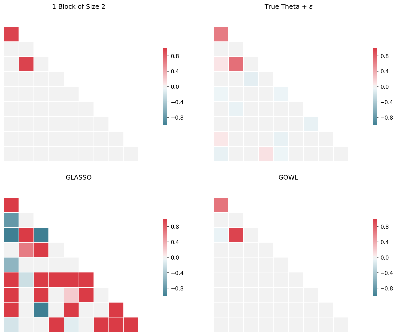
Here \(\Theta \in \mathbb{R}^{p \times p}\), \(\text{vechs}(\Theta)_{[i]}\) is the \(i^{th}\) largest off-diagonal component in magnitude of \(\Theta\), \(K = (p^2 - p)/2\), and \(\lambda_1 \ge \lambda_2 \ge \cdots \ge \lambda_p \ge 0\). The goal of this estimator is to identify correlated groups within the precision matrix estimator \(\hat{\Theta}\).

Synthetic Data Example

We design our first example for a very low \(p\) and specify one group of size two. As is custom in the literature we also standardize our design matrix \(X\).

p = 10
n = 100
n_blocks = 1
theta_star_eps, blocks, theta_star = generate_theta_star_gowl(p=p,
                                                              alpha=0.5,
                                                              noise=0.1,
                                                              n_blocks=n_blocks,
                                                              block_min_size=2,
                                                              block_max_size=6)

Hyperparameters should be chosen by cross-validation, but for this example we will choose \(\lambda_1 = 0.001\) and \(\lambda_2 = 0.01\). Now that we have generated \(\theta^*\) and \(\theta^* + \varepsilon\) we can generate a dataset by drawing i.i.d. from \(N(0, (\theta^* + \varepsilon)^{-1}\) distribution.

theta_star_eps = theta_star_eps[0]  # by default we generate 1 trial, but for simulations we generate many trials
sigma = np.linalg.inv(theta_star_eps)
n = 100
X = np.random.multivariate_normal(np.zeros(p), sigma, n)
X = standardize(X)  # Standardize data to have mean zero and unit variance.
S = np.cov(X.T)

lam1 = 0.001  # controls sparsity
lam2 = 0.01  # encourages equality of coefficients

Now that we have generated the dataset, we can apply the GOWL model using G-ISTA with backtracking line search enabled and duality gap stopping criteria.

model = GOWLModel(X, S, lam1, lam2, 'backtracking', max_iters=100000)
model.fit()
theta_gowl = model.theta_hat

iterations: 17
Duality Gap: -0.05034415853389618 < 1e-05. Exiting.

Let’s compare the GOWL theta estimate to the Graphical LASSO model.

gl = GraphicalLasso()
gl.fit(S)
theta_glasso = gl.get_precision()

plot_multiple_theta_matrices_2d([
    theta_star, theta_star_eps, theta_glasso, theta_gowl
], [
    f"1 Block of Size 2", 'True Theta + $\epsilon$', 'GLASSO', 'GOWL'
])